Peter Jennings
August, 2026
Tracking Ultrasonic Fish Tags
Tagged Fish
This is a continuation of the project I started in 2023 to follow the tagged fish in Ston(e)y Lake. In 2023, I built an ultrasonic detector that simply looked for 69KHz sounds in the water. This summer, I expanded that project to identify individual fish and investigate their habits.
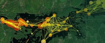 Dr Graham Raby and Dr Jake Brownscombe have an ongoing project to track the movement
of fish in Stony Lake using ultrasonic tracking transmitters surgically implanted into a number of captured and released fish. As of June, 2026, about 350 fish had been outfitted with transmitters provided by Innovasea.
Dr Graham Raby and Dr Jake Brownscombe have an ongoing project to track the movement
of fish in Stony Lake using ultrasonic tracking transmitters surgically implanted into a number of captured and released fish. As of June, 2026, about 350 fish had been outfitted with transmitters provided by Innovasea.
Innovasea uses three types of ID encoding on their tags. PPM (Pulse postion modulation) encodes information in the time intervals between 8 or 10 successive transmitted pulses or pings. HR (High Residency) encodes the ID as bits within a single millisecond transmission. HTI encodes the ID in the interval between successive pulses.
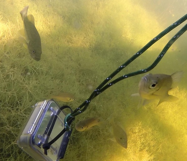
I was planning to build my own hydrophone and recorder when I came across the Hydromoth from Open Acoustic Devices. The AudioMoth, Hydromoth and MicroMoth were created by two computer science PhD students at the University of Southampton, Andrew Hill and Peter Prince, together with Alex Rogers, a computer science professor at the University of Oxford. The Hydromoth is an Audiomoth enclosed in a GoPro style underwater case. Unaccustomed as I am to buying something when I could build it myself, particularly when there is open source hardware and software to ease the journey, I decided to order one and save myself a lot of time.
The Audiomoth runs firmware on a EFM32 Gecko processor capable of recording uncompressed audio to a micro SD card from 8k to 384k samples/second in a WAV format. It runs on 3xAA batteries, which can be Alkaline, NiMH, or Lithium. It even has an onboard real-time clock to keeps track of the time.
I found that it works really well with Lithium rechargeable batteries so that battery life was never an issue. The 32GB SD card records several hours of audio in 90 minute chunks. The firmware provided even has a triggered mode that can turn on when it detects a 69 KHz signal, enabling many days of recording, albeit at the expense of missing some weak signals and often truncating the beginning of tag IDs.
As soon as we were settled into the cottage, I configured the Audiomoth to be triggered with a 69 KHz signal and, holding my breath, dropped it into the water, dangling on a line attached to our dock. I don't trust "waterproof" cases until I have seen them in the water for a while. I left it in the water overnight and hoped for the best.
Hydromoth Settings
The Hydromoth was dangled from our dock in about 2 meters of water. The case worked great. No water was ever found inside. The Hydromoth LED shows when it is recording, so it was easy to pull it up from time to time and check the status without opening. When convenient, the SD card was pulled and the data read.
Some experimentation was done on the settings but the first settings I used turned out to be pretty good for balancing detections against filling up the SD card too quickly with continuous recording. For the record, most of the time, the AudioMoth configuration was set to record at a sample rate of 384 KHz. High gain. Active: 24/7. Trigger frequency: 69 KHz. Trigger window: 32 samples. Record duration: 30 seconds. Each WAV file also includes the actual settings in the GUANO data.
Listening to the recorded audio, the first observation was that it was pretty noisy in the water. Boats starting and running could be heard almost constantly. Rain on the surface created underwater sounds. When there was any chop or the wind was blowing, there were sounds from boats rattling against their docks. Or moving around in our boathouse, which is where the acoustic receiver was located. How much do fish hear?
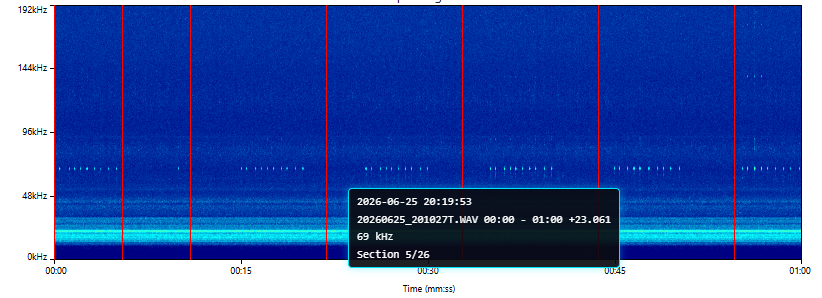
Open Acoustic Devices provides an excellent webapp, AudioMoth Play, which makes it super simple to look at the triggered WAV recording. I have added some features that I found useful, such as displaying the frequency and converting the triggered wave file times to real clock time. Both are open source under MIT License on github. See the bottom of the apps.
The results exceeded my expectations. I had hoped that maybe, if I was lucky, I would see something resembling a tag signal at some time during my 13 hours of listening. Looking at the spectrogram, it was clear that there were tag signals present immediately when I dropped the device into the water and that they displayed the timed pulse characteristic I was expecting. Now I know why so many fishermen show up in "our" bay.
Visual Tag Extraction
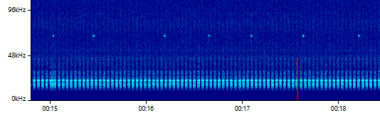
The play application allows dragging on the main spectrogram to zoom in on a section of audio.Visually, tags are easy to spot and a simple drag from beginning to end highlights the tag. Spotting tags visually this way is almost 100% accurate. Even partial tag reception jumps out of the spectrogram when the filters are adjusted for maximum visual contrast. I also experimented with converting the 69 KHz signal to audio at 400 Hz in order to listen to the tags. This also was a very reliable way to catch actual tags out of the noise. Our eyes and ears have very efficient algorithms for detecting patterns.

Thanks to the well documented Play application written by Alex and his team, it was possible to add a few lines of Javascript here and there to do some timing of the spaces between blips in milliseconds. After hand selecting a few hundred clean looking tags from the spectrogram and collecting the data a frequency analysis was done using Google Sheets. It soon became apparent that there were clear clusters every 20 mSec. This worked out very nicely as the minimum gap was 420 mSec and the maximum was 740 mSec (excluding some random exceptions). It looked like each gap could be reduced to a single hexadecimal digit. Tags with 10 blips produced a 9 digit hexadecimal ID. These were very common. Also showing up were 8 blip IDs with 7 gaps. And a random assortment of other patterns.
I was aware that many of the tags also carry sensor data but have no way to understand what that means in terms of signals. Probably those tags would not repeat as often as simple ID tags. But there is the possibility that what I identify as an ID is actually an ID combined with a sensor that is reading the same water temperature, depth, or fish acceleration. There is no way of knowing without more information.
Automated Tag Extraction
Although it was very accurate, it was not long before I tired of visually identifying tags and having the first iteration of the decoding software convert them into trains of gap times. It was time to begin a new app to automate the process. At this point Claude.ai became my programming staff and together we concocted a Tag Extractor program that is capable of analysing a wav file in a few seconds and reducing each found tag to a hexadecimal sequence.
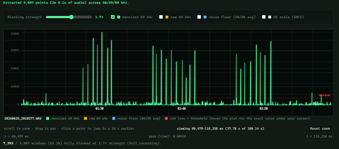
The Tag Extractor was set up to visualize the data with the option of an automatic threshold or a manuall override. First the wav signal was reduced to three channels of audio using the efficient Goertzel filters at 5 ms resolution. The prime channel at 69 KHz contains the tag signal. The secondary channels at 60 and 80 KHz contain the background noise. Often a sharp tap sound will produce a strong signal at almost all frequencies. Filtering it out of the data was the prime objective. The noise at 60 and 80 KHz was subtracted from the signal at 69 KHz to produce a clean output. An adjustable threshold modified by the noise around the sample time was used to determine what was signal and what was noise. Trial and error and some guesstimating resulted in the use of a threshold of 0.0004 of the full scale amplitude (68 dB below full scale ). As more data is accumulated, it would be possible to re-run the analysis and to create more efficient threshold computation. But for our purposes, this works pretty well.
Fixing Broken IDs
Examining the list of hexadecimal ID numbers, it was clear that many were typos of the most common IDs. 21683D9, 0F21F3D9, 21683D, were all probably inaccurate readings of tag 0F21683D9. A program was written to analyse the list of IDs and identify close IDs that were probably the result of late triggering, noise during the reception, or inaccurate timing of the gaps. A series of error correction algorithms were applied to fix these "broken" ID reports and reduce the number of probably "real" tag identifiers. A lot of trial and error and several iterations of the program led to the final automatic version which allows the incorporation of several days of new observations in a few minutes.
Tag Explorer
The Tag Explorer webapp was developed in parallel with the various extraction experiments to examine the resulting dataset, which was the goal of the whole project. Every day, I would wake up with a new idea to incorporate into the visual dashboard for examining the habits of my visiting fish. Thanks to Claude's efficient programming, these ideas could be incorporated remarkably quickly into the growing page. Like many other apps, adding features in a haphazard manner makes it less friendly and prone to bugs. I don't generally recommend it.
You are welcome to play with the Tag Explorer using the collected data.
If you have any data of your own in a simple csv file containing the date time,signal strength,ID\n
on each line, then all of the features are available.
The data is entirely analysed in the browser. Nothing is uploaded to my servers.
There is a complete
User Manual to explain the operation of each of the
panels. Both the User Manual and the Tag Explorer tool can be displayed in dark or
light mode according to your preference. Tap the icon at the top right.
Most functions have direct references to the User Manual. Click the
 icon.
icon.
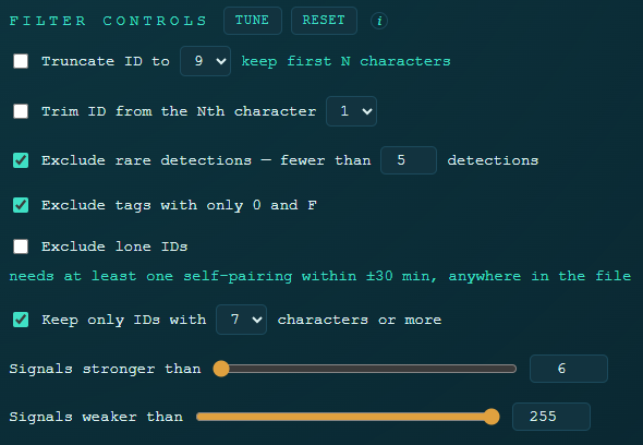
Rather than discarding the noisy detections, all of the possible fish tag data is available for analysis. To reduce the noise, the filters allow the exclusion of random partial tags and noise interpreted as being part of a tag. Click to view all the data. Click for a set of preset filters that I like to use. The filters were useful in the earlier stages when developing the error correction algorithms.
It is also possible to exclude strong or weak signals with the sliders.
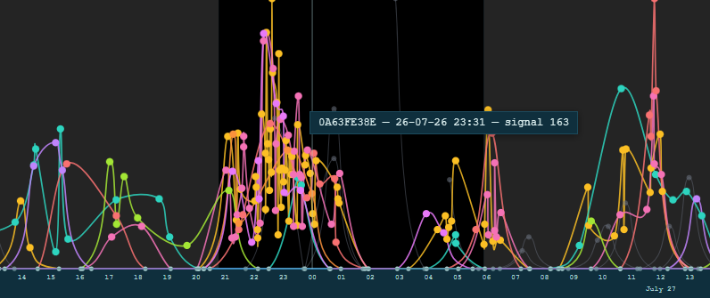
The signal strength plot shows the received signal power of each identified fish over time. The plot can be zoomed in and out and panned. Clicking on any data point narrows the display to just that fish. The zoomed in pattern of signal strength showing a fish approaching the detector and moving away in a regular pattern confirms that the data collected is reasonable. Double click restores the plot to the full date range of the data.
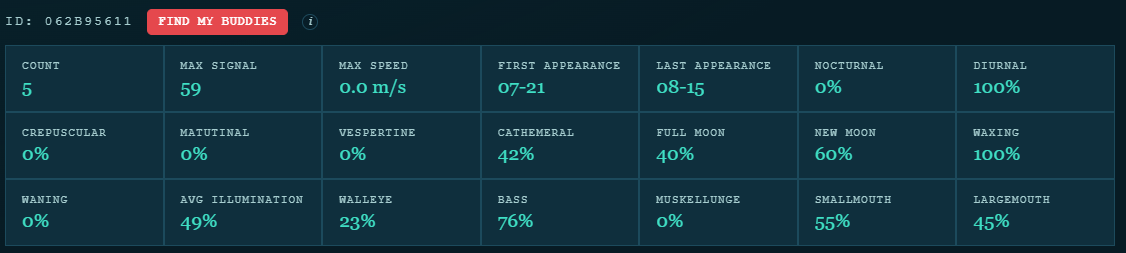
When a single fish is selected, the information about that fish is displayed in a panel below the plot. The button restricts the list to fish that are seen at the same time as the one selected.
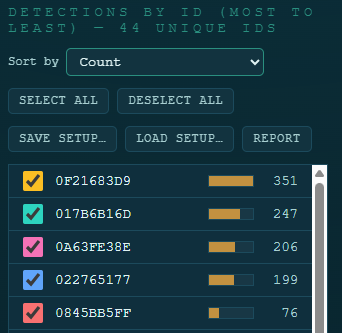
At the left is a checkbox list of all the IDs that made it through the filters and selections. The top 10 are coloured and match the colours on the signal strength plot.
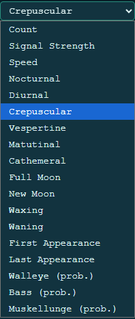
The sort pulldown lets you sort the list by various parameters based on the detections. Speed is calculated from the fastest rate of change of the signal. Time of day calculations are based on actual sunrise and sunset times. Time of the moon cycle were included for the fun of it. A set of heuristics was used to determine the probability that the fish is a muskie, walleye, or bass, based on when they appeared in the data and their calculated speed.
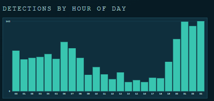
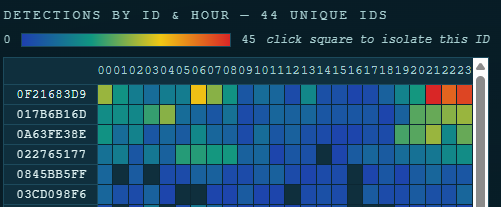
The histograms and heatmaps show various detection frequencies. They all show more information on a mouse hover. Clicking affects the checklist and shows only the fish that are present in each statistic. For example, clicking on hour 17 restricts the display to only the fish that were present in that hour on some day. The plot will now show just those selected fish at other times and on other days.
Click above the checkboxes to restore the full selection.
General Observations
All of this has to be taken with a grain of salt. There was no attempt at scientific rigour. Trigger and extraction threshold parameters varied during the study. The hydromoth was not always operating (off periods are marked in red on the plot). The number of detections is probably not statistically significant. The error correction fixes could lead to false identifications. And so on. For me, the fun was in developing the software and playing with the data.
The temperature data is only for the summer. The temperature sensor is near the surface. Our bay warms up a lot when the sun is shining. It also cools quickly when it rains. The temperature histogram probably reflects the day and time more than any actual correlation between temperature and fish counts.
The heuristics indicate that Walleye are regularly hanging around in the bay. You are 10 times more likely to see one at 10 at night than at 4 in the afternoon. Of course, they might be here, but they might not be hungry. This may be where the hang out when they aren't looking for food, so it might not be useful information for fishermen.
- Tag Explorer. The data exploration tool you can use to play with the data. Come to your own conclusions.
- User Manual. The guide to the various tools in the Tag Explorer with some elucidation of the methods used.
- References. The reference guide with more detailed descriptions of the methods used in the extraction process and the explorer. Includes footnotes and references to the origins of the methods and algorithms.
Ideas for further experimentation
I hope the batteries in the fish transmitters will last long enough for me to try some of these ideas next summer.
Keeping track of other parameters such as actual sunlight brightness on the water, minute by minute, or wind direction and speed, would make for an interesting analysis. Do the fish seek shelter in our shallow bay, or avoid it, depending on the conditions?
The Audiomoth can be configured as an ultrasonic microphone. I have already tested and proved it works with the Android BatRecorder App, which is now free and open source. The next step is to waterproof the microphone and go looking for fish. Since the detector app is open source, it should be possible to extend it to decode the tags in real time.
Placing multiple Hydromoths around the bay and synchronizing the timing should give a 3D location of the fish. Doing this with a mesh of connected Android devices would give real time location information. Fun, but a bigger investment.
When the data is collected from the receivers in the centre of the bay, it will be possible to correlate the true IDs with mine. It will be interesting to see how my heuristic fish identifications compare with the actual tagged fish. Let's hope that they are willing to share some files.
Since the AudioMoth firmware is open source, it should be quite straightforward to incorporate some of the tag decoding. Saving only the tag information would reduce the SD card requirements. Battery life is estimated to be several months with Lithium AA batteries. More data = more fun.
A Hydromoth can be connected to a GoPro or other underwater camera and short videos can be triggered by a strong tag detection. An actual image of the visiting fish would be possible. The products I designed for CamDo Solutions Inc 15 years ago to trigger the camera and underwater WiFi would be perfect.
What ideas do you have? I am always open to suggestions. Do you have questions that the data might already answer? The entire Tag Explorer app is one html file with Javascript. Download it and give it to Claude. Claude can modify it to answer your question. ...sometimes.